Introduction
If your data is noisy, you may need to apply a smoothing algorithm to expose its features and to provide a reasonable starting approach for parametric fitting. The two basic assumptions that underlie smoothing are:
- The relationship between the response data and the predictor data is smooth.
-
The smoothing process results in a smoothed value that is a better estimate of the original value because the noise has been reduced.
The smoothing process attempts to estimate the average of the distribution of each response value. The estimation is based on a specified number of neighboring response values.
You can think of smoothing as a local fit since a new response value is created for each original response value. Therefore, smoothing is similar to some of the nonparametric fit types supported by the tool such as smoothing spline and cubic interpolation. However, this type of fitting is not the same as parametric fitting, which results in a global parameterization of the data.
There are two common types of smoothing methods: filtering (averaging) and local regression. Each smoothing method requires a span. The span defines a window of neighboring points to include in the smoothing calculation for each data point. This window moves across the data set as the smoothed response value is calculated for each predictor value. A large span increases the smoothness but decreases the resolution of the smoothed data set, while a small span decreases the smoothness but increases the resolution of the smoothed data set. The optimal span value depends on your data set and the smoothing method, and usually requires some experimentation to find.
The Curve Fitting Tool supports these smoothing methods:
- Moving average filtering – Lowpass filter that takes the average of neighboring data points.
- Lowess and loess – Locally weighted scatter plot smooth. These methods use linear least squares fitting and a first degree polynomial (lowess) or a second degree polynomial (loess). Robust lowess and loess methods that are resistant to outliers are also available.
- Savitzky-Golay filtering – A generalized moving average where the filter coefficients are derived by performing an unweighted linear least squares fit using a polynomial of a given degree.
You smooth data with the Smooth tab of the Data GUI.
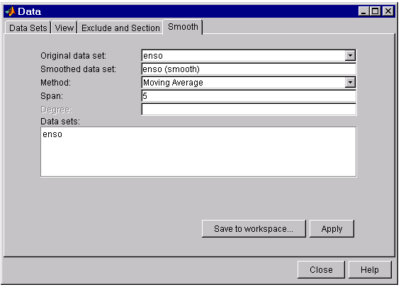
The fields are described below:
- Original data set – Select the data set you want to smooth.
- Smoothed data set – Specify the name of the smoothed data set. Note that the process of smoothing the original data set always produces a new data set containing smoothed response values.
- Method – Select the smoothing method. Each response value is replaced with a smoothed value that is calculated by the specified smoothing method:
- Moving average – Filter the data by calculating an average.
- Lowess – Locally weighted scatter plot smooth using linear least squares fitting and a first degree polynomial.
- Loess – Locally weighted scatter plot smooth using linear least squares fitting and a second degree polynomial.
- Savitzky-Golay – Filter the data using a polynomial of the specified degree.
- Robust Lowess – Lowess method that is resistant to outliers.
- Robust Loess – Loess method that is resistant to outliers.
-
Span – The number of data points used to compute each smoothed value.
For the moving average and Savitzky-Golay methods, the span must be odd. If you specify an even span an error is returned. For the robust and nonrobust lowess and loess methods, if the span is less than 1, it is interpreted as the percentage of the total number of data points.
- Degree – The degree of the polynomial used in the Savitzky-Golay method. The degree must be smaller than the span.
- Data sets – Lists all the original and smoothed data sets.
Moving average filtering
A moving average filter smooths data by replacing each data point with the average of the neighboring data points defined within the span. This process is equivalent to lowpass filtering with the response of the smoothing given by the difference equation:
\[y_{s}(i) = {1\over{2N+1}}{\left(y(i+N)+y(i+N-1)+...+y(i-N)\right)}\]where \(y_{s}(i)\) is the smoothed value for the \(ith\) data point, N is the number of neighboring data points on either side of \(y_{s}(i)\), and \(2N+1\) is the span.
The moving average smoothing method used by the Curve Fitting Tool follows these rules:
- The span must be odd.
- The data point to be smoothed must be at the center of the span.
- The span is adjusted for data points that cannot accommodate the specified number of neighbors on either side.
- The end points are not smoothed since a span cannot be defined.
For example, suppose you smooth data using a moving average filter with a span of 5. Using the rules described above, the first four elements of ys are given by
\(y_{s}(1) = y(1)\)
\(y_{s}(2) = (y(1)+y(2)+y(3))/3\)
\(y_{s}(3) = (y(1)+y(2)+y(3)+y(4)+y(5))/5\)
\(y_{s}(4) = (y(2)+y(3)+y(4)+y(5)+y(6))/5\)
Note that \(y_{s}(1), y_{s}(2), ... ,y_{s}(end)\) refers to the order of the data after sorting, and not necessarily the original order.
The smoothed values and spans for the first four data points of a generated data set are shown below.
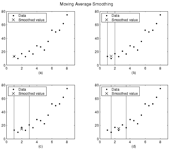
Plot (a) indicates that the first data point is not smoothed since a span cannot be constructed. Plot (b) indicates that the second data point is smoothed using a span of three. Plots (c) and (d) indicate that a span of five is used to calculate the smoothed value.
Lowess and loess
You perform local regression smoothing with the lowess and loess methods. The names “lowess” and “loess” are derived from the term “locally weighted scatter plot smooth” since both methods use locally weighted linear regression to smooth data.
The smoothing process is considered local since, like the moving average method, each smoothed value is determined by neighboring data points defined within the span. The process is weighted since a regression weight function is defined for the data points contained within the span. In addition to the regression weight function, you can use a robust weight function, which makes the process resistant to outliers. Finally, the methods are differentiated by the model used in the regression; lowess uses a linear polynomial and loess uses a quadratic polynomial.
The local regression smoothing methods used by the Curve Fitting Tool follow these rules:
- The span can be even or odd.
- You can specify the span as a percentage of the total number of data points in the data set. For example, a span of 0.1 uses 10% of the data points.
The regression smoothing and robust smoothing procedures are described in detail below.
Smoothing procedure
The local regression smoothing process follows these steps for each data point:
-
Compute the regression weights for each data point in the span. The weights are given by the bicube function:
\[w_{i} = \left(1 - {\left|(x - x_{i}) \over d(x)\right|}^3 \right)^3\]\(x\) is the predictor value associated with the response value to be smoothed, \(x_{i}\) are the nearest neighbors of \(x\) as defined by the span, and \(d(x)\) is the distance from \(x\) to the most distant predictor value within the span.
- A weighted linear least squares regression is performed. For lowess, the regression uses a first degree polynomial. For loess, the regression uses a second degree polynomial.
- The smoothed value is given by the weighted regression at the predictor value of interest.
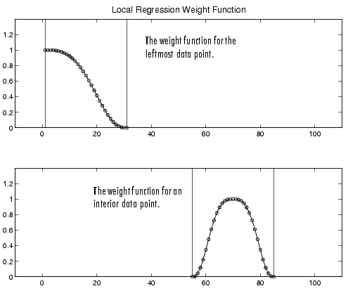
If the smooth calculation involves the same number of neighboring data points on either side of the smoothed data point, then the weight function is symmetric. However, if the number of neighboring points is not symmetric about the smoothed data point, then the weight function is not symmetric. Note that unlike the moving average smoothing process, the span never changes. For example, when smoothing the data point with the smallest predictor value, the shape of the weight function is truncated by one half, the leftmost data point in the span has the largest weight, and all the neighboring points are to the right of the smoothed value.
The weight function for an end point and for an interior point is shown below for a span of 31 data points.
Using the lowess method with a span of five, the smoothed value and associated regression for the first four data points of a generated data set are shown below.
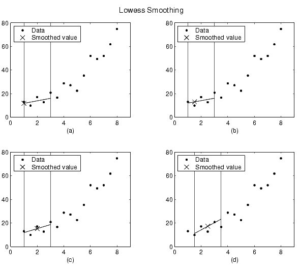
Notice that the span does not change as the smoothing process progresses from data point to data point. However, depending on the number of nearest neighbors, the regression weight function may not be symmetric about the data point to be smoothed. In particular, plots (a) and (b) use an asymmetric weight function, while plots (c) and (d) use a symmetric weight function.
For the loess method, the graphs would look the same except the smoothed value would be generated by a second degree polynomial.
Robust smoothing procedure
If your data contains outliers, then the smoothed values can become distorted and not reflect the behavior of the bulk of the neighboring data points. To overcome this problem, you can smooth the data using a robust procedure that is not influenced by a small fraction of outliers.
The Curve Fitting Tool provides a robust version for both the lowess and loess smoothing methods. These robust methods include an additional calculation of robust weights, which is resistant to outliers. The robust smoothing procedure follows these steps:
- Calculate the residuals from the smoothing procedure described previously.
-
Compute the robust weights for each data point in the span. The weights are given by the bisquare function shown below.
\[w_{i} = \begin{cases} \left(1 - (r_{i} / 6MAD)^2 \right)^2 & \left|r_{i}\right| \lt 6MAD \\ 0 & \left|r_{i}\right| \ge 6MAD \end{cases}\]\(r_{i}\) is the residual of the \(ith\) data point produced by the regression smoothing procedure, and \(MAD\) is the median absolute deviation of the residuals
\[MAD = median(|r|)\]The median absolute deviation is a measure of how spread out the residuals are. If \(r_{i}\) is small compared to \(6MAD\), then the robust weight is close to 1. If \(r_{i}\) is greater than \(6MAD\), the robust weight is 0 and the associated data point is excluded from the smooth calculation.
-
Smooth the data again using the robust weights. The final smoothed value is calculated using both the local regression weight and the robust weight.
- Repeat the previous two steps for a total of five iterations.
The smoothing results of the lowess procedure are compared below to the results of the robust lowess procedure for a generated data set that contains a single outlier. The span for both procedures is 11 data points.
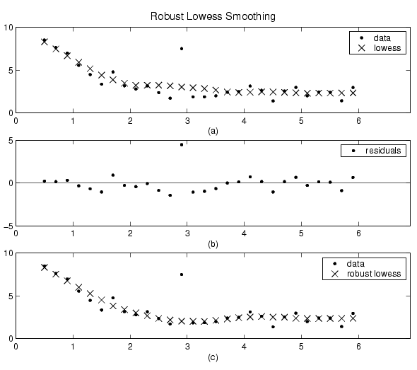
Plot (a) shows that the outlier influences the smoothed value for several nearest neighbors. Plot (b) suggests that the residual of the outlier is greater than six median absolute deviations. Therefore, the robust weight is zero for this data point. Plot (c) shows that the smoothed values neighboring the outlier reflect the bulk of the data.
Savitzky-Golay filtering
Savitzky-Golay filtering is a generalized moving average. The filter coefficients are derived by performing an unweighted linear least squares fit using a polynomial of a given degree. For this reason, a Savitzky-Golay filter is also called a digital smoothing polynomial filter or a least squares smoothing filter. Note that a higher degree polynomial makes it possible to achieve a high level of smoothing without attenuation of data features.
The Savitzky-Golay filtering method is often used with frequency data or with spectroscopic (peak) data. For frequency data the method is effective at preserving the high frequency components of the signal. For spectroscopic data the method is effective at preserving higher moments of the peak such as the line width. By comparison, the moving average filter tends to filter out a significant portion of the signal’s high frequency content, and it can only preserve the lower moments of a peak such as the centroid. However, Savitzky-Golay filtering can be less successful than a moving average filter at rejecting noise.
The Savitzky-Golay smoothing method used by the Curve Fitting Tool follows these rules:
- The span must be odd.
- The polynomial degree must be less than the span.
-
The data points are not required to have uniform spacing.
Normally, Savitzky-Golay filtering requires uniform spacing of the predictor data. However, the algorithm provided by the Curve Fitting Tool supports nonuniform spacing. Therefore, you are not required to perform an additional filtering step to create data with uniform spacing.
The plot shown below displays generated Gaussian data and several attempts at smoothing using the Savitzky-Golay method. The data is very noisy and the peak widths vary from broad to narrow. The span is equal to 5% of the number of data points.
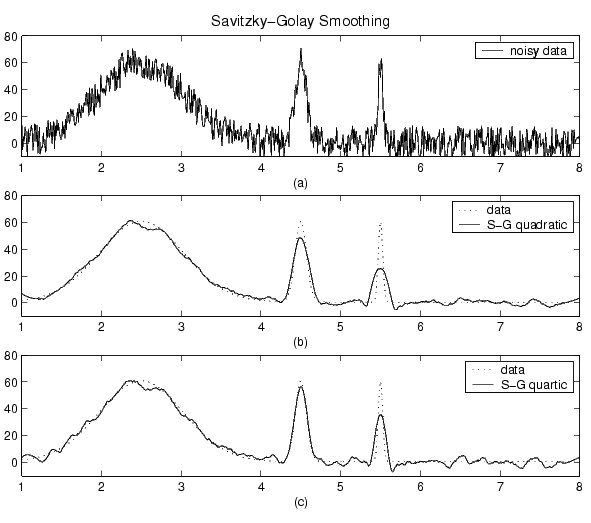
Plot (a) shows the noisy data. To more easily compare the smoothed results, plots (b) and (c) show the data without the added noise. Plot (b) shows the result of smoothing with a quadratic polynomial. Notice that the method performs poorly for the narrow peaks. Plot (c) shows the result of smoothing with a quartic polynomial. In general, higher degree polynomials can more accurately capture the height and widths of narrow peaks, but can do poorly at smoothing wider peaks.
Example: Smoothing data
This example smooths the ENSO data set using the moving average, lowess, loess, and Savitzky-Golay methods with the default span. As shown below, the data appears noisy. Smoothing may help you visualize patterns in the data, and provide insight toward a reasonable approach for parametric fitting.
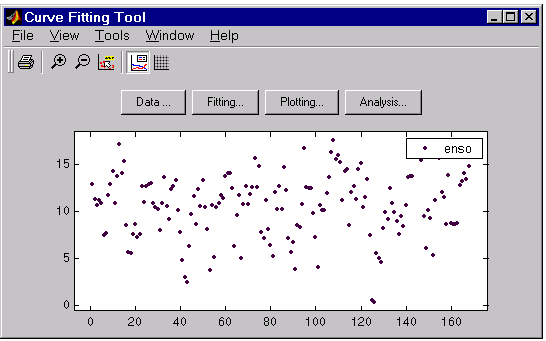
The Smooth tab shown below displays all the new data sets generated by smoothing the original ENSO data set. Whenever you smooth a data set, a new data set of smoothed values is created.
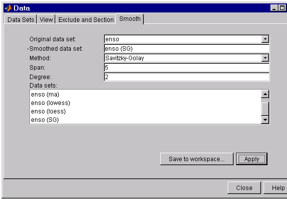
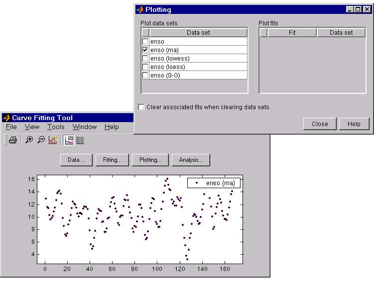
The smoothed data sets are automatically displayed in the Curve Fitting Tool. Use the Plotting GUI to display only the data sets of interest.
As shown below, the periodic structure of the ENSO data set becomes apparent when it is smoothed using a moving average filter with the default span. Not surprisingly, the uncovered structure is periodic, which suggests that a reasonable parametric model should include trigonometric functions.
Saving the results
Press the Save to workspace button to save a smoothed data set as a structure to the workspace. This example saves the moving average results contained in the enso (ma) data set.

The saved structure contains the original predictor data x, and the smoothed data y.
smootheddata1

smootheddata1 =
    x: [168x1 double]
    y: [168x1 double]