Introduction
Parametric fitting involves finding coefficients (parameters) for one or more models that you fit to data. The data is assumed to be statistical in nature and is divided into a deterministic component and a random component.
\[\text{data = deterministic component + random component}\]The deterministic component is given by the fit and the random component is the error associated with the data.
\[\text{data = fit + error}\]The fit is given by a model that is a function of the independent (predictor) variable and one or more coefficients. The error represents random variations in the data that follow a specific probability distribution (usually Gaussian). The variations can come from many different sources, but are always present at some level when dealing with measured data. Systematic variations may also exist, but they can be difficult to quantify.
The fitted coefficients often have physical significance. For example, suppose you have collected data that corresponds to a single decay mode of a radioactive nuclide, and you want to find the half-life (T1/2) of the decay. The law of radioactive decay states that the activity of a radioactive substance decays exponentially in time. Therefore, the model to use in the fit is given by:
\[y = y_{0}e^{-\lambda t}\]where \(y_{0}\) is the number of nuclei at time t = 0, and \(\lambda\) is the decay constant. Therefore, the data can be described by:
\[\text{data} = y_{0}e^{-\lambda t} + \text{error}\]Both \(y_{0}\) and \(\lambda\) are coefficients returned by the fit. Since \(T_{1/2} = ln(2)/\lambda\), the fitted value of the decay constant yields the half-life. However, since the data contains some error, the deterministic component of the equation cannot completely describe the variability in the data. Therefore, the coefficients and half-life calculation will have some uncertainty associated with them. If the uncertainty is acceptable, then you are done fitting the data. If the uncertainty is not acceptable, then you may have to take steps to reduce the error and repeat the data collection process.
Assumptions about the error
When fitting data that contains random variations, there are two core assumptions that are usually made about the error:
- The error exists only in the response data, and not in the predictor data.
- The errors are random and follow a normal (Gaussian) distribution with zero mean and constant variance, \(\sigma^{2}\)2.
The second assumption is often expressed as:
\[\text{error} \sim N(0,\sigma^{2})\]The components of this expression are described below.
- Normal distribution – The errors are assumed to be normally distributed because the normal distribution often provides an adequate approximation to the distribution of measured quantities. Although the least squares fitting method does not assume normally distributed errors when calculating parameter estimates, the method works best for data that does not contain a large number of random errors with extreme values. The normal distribution is one of the probability distributions in which extreme random errors are uncommon. However, statistical results such as confidence and prediction bounds do require normally distributed errors for their validity.
- Zero mean – If the mean of the errors is zero, then the errors are purely random. If the mean is not zero, then the model may not be the right choice for your data, or the errors are not purely random and contain systematic errors.
-
Constant variance – A constant variance in the data implies that the “spread” of errors is constant. Data that has the same variance is sometimes said to be of equal quality.
The assumption that the random errors have constant variance is not implicit to weighted least squares regression. Instead, it is assumed that the weights provided in the fitting procedure correctly indicate the differing levels of quality present in the data. The weights are then used to adjust the amount of influence each data point has on the estimates of the fitted coefficients to an appropriate level.
Library models
The parametric library models provided by the Curve Fitting Tool are described below.
Exponentials
Exponentials are often used when the rate of change of a quantity is proportional to the initial amount of the quantity. The tool provides a one-term and a two-term exponential model:
\[y = ae^{bx}\] \[y = ae^{bx} + ce^{dx}\]If the coefficient associated with the exponent is negative, then \(y\) represents exponential decay. For example, a single radioactive decay mode of a nuclide is described by a one-term exponential where \(a\) is the initial number of nuclei, \(b\) is the decay constant, \(x\) is time, and \(y\) is the number of remaining nuclei after a specific amount of time passes. If two decay modes exist, then you must use the two-term exponential model.
If the coefficient associated with the exponent is positive, then \(y\) represents exponential growth. Examples of exponential growth include contagious diseases for which a cure is unavailable, and biological populations whose growth is uninhibited by predation, environmental factors, and so on.
Fourier series
The Fourier series is a sum of sine and cosine functions that is used to describe periodic data. It is represented in either the trigonometric form or the exponential form. The tool provides the trigonometric form:
\[y = a_{0} + \sum_{i=1}^{n}{a_{i}cos(nwx) + b_{i}sin(nwx)}\]where \(a_{0}\) models any DC offset in the data and is associated with the \(i = 0\) cosine term, \(w\) is the fundamental frequency of the data, and \(n\) is the number of terms (harmonics) in the series.
Gaussian
The Gaussian model is used for fitting peaks and is given by:
\[y = \sum_{i=1}^{n}{ a_{i}e^{ -\left(x - b_{i}\over c_{i} \right) ^2}}\]where \(a\) is the amplitude, \(b\) is the centroid (location), \(c\) is related to the peak width, \(n\) is the number of peaks to fit, and \(1 \le n \le 8\).
Gaussian peaks are encountered in many areas of science and engineering such as line emission spectra and chemical concentration assays.
Polynomials
Polynomials are often used when a simple empirical model is required. The model may be used for interpolation or extrapolation, or it may be used to characterize data using a global fit. For example, the temperature-to-voltage conversion for a Type J thermocouple in the \(0^{o}\) to \(760^{o}\) temperature range is described by a seventh degree polynomial. Polynomial models are given by:
\[y = \sum_{i=1}^{n+1}{ p_{i}x^{n+1-i} }\]where \(n + 1\) is the order of the polynomial, \(n\) is the degree of the polynomial, and \(1 \le n \le 9\). The order gives the number of coefficients to be fit, and the degree gives the highest power of the predictor variable.
In this guide, polynomials are described in terms of their degree. For example, a third degree (cubic) polynomial is given by:
\[y = p_{1}x^{3} + p_{2}x^{2} + p_{3}x + p_{4}\]If you do not require a global parametric fit and want to maximize the flexibility of the fit, piecewise polynomials may provide the best approach.
The main advantages of polynomial fits include reasonable flexibility for data that is not too complicated, and they are linear, which means the fitting process is simple. The main disadvantage is that high degree fits can become unstable. Additionally, polynomials of any degree can provide a good fit within the data range, but may diverge wildly outside that range. Therefore, you should exercise caution when extrapolating with polynomials.
When you fit with high degree polynomials, the fitting procedure uses the predictor values as the basis for a matrix with very large values, which can result in scaling problems. To deal with this, you should normalize the data by centering it at zero mean and scaling it to unit standard deviation. You normalize data with the Center and scale X data check box on the Fitting GUI.
Power series
Power series models are used to describe a variety of data. For example, the rate at which reactants are consumed in a chemical reaction is generally proportional to the concentration of the reactant raised to some power. The tool provides a one-term and a two-term power series model:
\[y = ax^{b}\] \[y = a + bx^{c}\]Rationals
Like polynomials, rationals are often used when a simple empirical model is required. The main advantage of rationals is their flexibility with data that has complicated structure. The main disadvantage is that they become unstable when the denominator is around zero. Rational models are defined as ratios of polynomials:
\[y = {\sum_{i=1}^{n+1}{p_{i}x^{n + 1 - i}} \over x^{m} + \sum_{i=1}^{m}{q_{i}x^{m - i}}}\]where \(n\) is the degree of the numerator polynomial and \(1 \le n \le 5\), while \(m\) is the degree of the denominator polynomial and \(1 \le m \le 5\). Note that the coefficient associated with \(x^{m}\) is always 1, which makes the numerator and denominator unique when the polynomial degrees are the same.
In this guide, rationals are described in terms of the degree of the numerator / the degree of the denominator. For example, a quadratic/cubic rational equation is given by:
\[y = { p_{1}x^{2} + p_{2}x + p_{3} \over x^{3} + q_{1}x^{2} + q_{2}x + q_{3} }\]Sum of sines
The sum of sines model is used for fitting periodic functions. It is closely related to the Fourier series described previously, except it includes phase information and does not include a DC offset term. The sum of sines equation is given by:
\[y = \sum_{i=1}^{n}{ a_{i}sin(b_{i}x + c_{i}) }\]where \(a\) is the amplitude, \(b\) is the frequency, \(c\) is the phase for each sine wave term, and \(n\) is the number of terms in the series where \(1 \le n \le 8\).
Weibull distribution
The Weibull distribution is widely used in reliability and life (failure rate) data analysis. The tool provides the two-parameter Weibull distribution:
\[y = abx^{b - 1}e^{-ax^{b}}\]where \(a\) is the scale parameter and \(b\) is the shape parameter. Note that there is also a three-parameter Weibull distribution with \(x\) replaced by \(x - c\) where \(c\) is the location parameter. Additionally, there is a one-parameter Weibull distribution where the shape parameter is fixed and only the scale parameter is fitted. To use these distributions, create a custom equation.
The Curve Fitting Tool does not fit Weibull probability distributions to a sample of data. Instead, it fits curves to response and predictor data such that the curve has the same shape as a Weibull distribution.
Custom equations
If the library does not contain the desired parametric equation, then you must create your own custom equation. However, you should use the library equations if possible since they offer the best chance for rapid convergence because:
- For most models, optimal default coefficient starting points are calculated. For custom equations, the default starting points are chosen at random on the interval [0,1].
- An analytic Jacobian is used instead of finite differencing.
- When using the Analysis GUI, analytic derivatives are calculated as well as analytic integrals if the integral can be expressed in closed form.
You create custom equations with the Create Custom Equation GUI. The GUI contains a tab for creating linear equations and a tab for creating general (nonlinear) equations.
Linear equations
Linear equations are defined as equations that are linear in the parameters. For example, the polynomial library equations are linear. The Linear equations tab is shown below followed by a description of the fields:
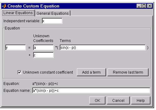
- Independent variable – Symbol representing the independent (predictor) variable. The default is
x. - Equation – Symbol representing the dependent (response) variable followed by the linear equation. The default is
y.- Unknown Coefficients – The unknown coefficients to be determined by the fit. The defaults are
a, b, c, .... - Terms – Functions that depend only on the predictor variable and constants. Note that if you attempt to define a term that contains a coefficient to be fitted, then an error is returned.
- Unknown constant coefficient – If checked, then a constant term is included in the equations to be fit. If not checked, then a constant term is not included.
- Add a term – Add a term to the equation. An unknown coefficient is automatically added for each new term.
- Remove last term – Remove the last term added to the equation.
- Unknown Coefficients – The unknown coefficients to be determined by the fit. The defaults are
- Equation – The custom equation.
- Equation name – By default, the name is automatically updated to be identical to the custom equation given by Equation. If you override the default, then the name is no longer automatically updated.
General equations
General (nonlinear) equations are defined as equations that are nonlinear in the parameters, or are a combination of linear and nonlinear in the parameters. For example, the exponential library equations are nonlinear. The General Equations tab is shown below followed by a description of the fields:
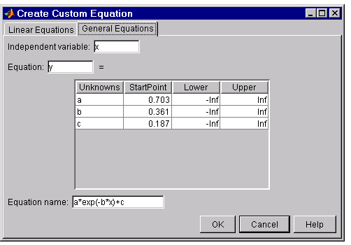
- Independent variable – Symbol representing the independent (predictor) variable. The default is
x. -
Equation – Symbol representing the dependent (response) variable followed by the general equation. As you type in the terms of the equation, the unknown coefficients, associated starting values, and constraints automatically populate the table. By default, the starting values are randomly selected on the interval [0,1] and are unconstrained.
You can change the default starting values and constraints in this table, or you can change them later using the Fit Options GUI.
- Equation name – By default, the name is automatically updated to be identical to the custom equation given by Equation. If you override the default, then the name is no longer automatically updated.
Note that even if you define a linear equation, a nonlinear fitting procedure will still be used. Although this is allowed by the tool, it is an inefficient process and may result in less than optimal fitted coefficients. In this case, you should use the Linear Equations tab instead.
Specifying fit options
You specify fit options with the Fit Options GUI. The fit options for the single-term exponential are shown below. The coefficient starting values and constraints are for the census data.
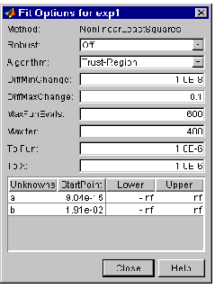
The available fields depend on the whether you are using a linear model, a nonlinear model, or a nonparametric fit type. The complete list of fields is given below:
-
Method – The fitting method.
The method is automatically selected based on the library or custom model you use. For linear models, the method is
LinearLeastSquares. For nonlinear models, the method isNonlinearLeastSquares. - Robust – Specify whether to use the robust least squares fitting method. The values are:
- Off – Do not use robust fitting (default).
- On – Fit with default robust method (bisquare weights).
- LAR – Fit by minimizing the least absolute residuals (LAR).
- Bisquare – Fit by minimizing the summed square of the residuals and downweight outliers using bisquare weights. In most cases, this is the best choice for robust fitting.
- Algorithm – Algorithm used for the fitting procedure:
- Trust-Region – This is the default algorithm and must be used if you specify coefficient constraints.
- Levenberg-Marquardt – If the trust-region algorithm does not produce a reasonable fit, and you do not have coefficient constraints, you should try the Levenberg-Marquardt algorithm.
- Gauss-Newton – This algorithm is included for pedagogical reasons and should be the last choice for most models and data sets.
- DiffMinChange – Minimum change in coefficients for finite difference Jacobians. The default value is \(10^{-8}\).
- DiffMaxChange – Maximum change in coefficients for finite difference Jacobians. The default value is
0.1. - MaxFunEvals – Maximum number of function (model) evaluations allowed. The default value is
600. - MaxIter – Maximum number of fit iterations allowed. The default value is
400. - TolFun – Termination tolerance used on stopping conditions involving the function (model) value. The default value is \(10^{-6}\).
- TolX – Termination tolerance used on stopping conditions involving the coefficients. The default value is \(10^{-6}\).
- Unknowns – Symbols for the unknown coefficients to be fitted.
- StartPoint – The coefficient starting values. The default values depend on the model. For rational, Weibull, and custom models, default values are randomly selected within the range [0,1]. For all other nonlinear library models, the starting values depend on the data set and are calculated heuristically.
- Lower – Lower bounds on the fitted coefficients. The bounds are used only with the trust region fitting algorithm. The default lower bounds for most library models are -Inf, which indicates that the coefficients are unconstrained. However, a few models have finite default lower bounds. For example, Gaussians have the width parameter constrained so that it cannot be less than 0.
- Upper – Upper bounds on the fitted coefficients. The bounds are used only with the trust region fitting algorithm. The default upper bounds for all library models are Inf, which indicates that the coefficients are unconstrained.
Default coefficient parameters
The default coefficient starting points and constraints for library and custom models are given below. If the starting points are optimized, then they are calculated heuristically based on the current data set. Random starting points are defined on the interval [0,1] and linear models do not require starting points.
If a model does not have constraints, then the coefficients have neither a lower bound or an upper bound. You can override the default starting points and constraints by providing your own values using the Fit Options GUI.
| Model | Starting Points | Constraints |
| Custom linear | N/A | none |
| Custom nonlinear | random | none |
| Exponentials | optimized | none |
| Fourier series | optimized | none |
| Gaussians | optimized | \(\text c_{i}\) > 0 |
| Polynomials | N/A | none |
| Power series | optimized | none |
| Rationals | random | none |
| Sum of sines | optimized | \(\text b_{i}\) > 0 |
| Weibull | random | a, b > 0 |
Note that the sum of sines and Fourier series models are particularly sensitive to starting points, and the optimized values may be accurate for only a few terms in the associated equations.
Example: Rational fit
This example fits measured data using a rational model. The data describes the coefficient of thermal expansion for copper as a function of temperature in degrees Kelvin. To get started, load the data from the hahn1 file.
load hahn1
The workspace contains two new variables:
tempis a vector of temperatures in degrees Kelvin.thermexis a vector of thermal expansion coefficients for copper.
For this data set you will find the rational equation that produces the best fit. Rational models are defined as a ratio of polynomials:
\[y = { p_{1}x^{n} + p_{2}x^{n-1} + ... + p_{n+1} \over x^{m} + q_{1}x^{m-1} + ... + q_{m} }\]where \(n\) is the degree of the numerator polynomial and \(m\) is the degree of the denominator polynomial. Note that the rational equations are not associated with physical parameters of the data. Instead, they provide a simple and flexible empirical model that you can use for interpolation and extrapolation.
By examining the shape of the data, a reasonable first choice is quadratic/quadratic:
\[y = { p_{1}x^{2} + p_{2}x + p_{3} \over x^{2} + q_{1}x + q_{2} }\]The Fit Editor configured for this equation is shown below.
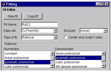
The data, fit, and residuals are shown below.
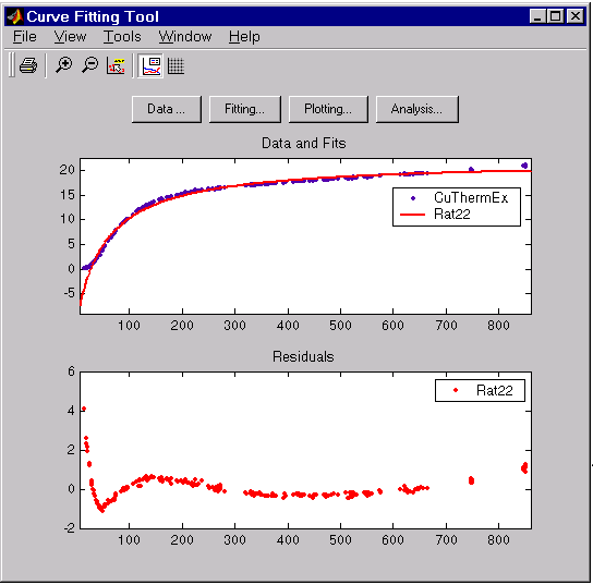
The fit clearly misses the data for the smallest and largest predictor values. Additionally, the residuals show a strong pattern throughout the entire data set indicating that a better fit is possible.
For the next fit, try a cubic/cubic equation:
\[y = {p_{1}x^{3} + p_{2}x^{2} + p_{3}x + p_{4} \over x^{3} + q_{1}x^{2} + q_{2}x + q_{3} }\]The data, fit, and residuals are shown below.

The numerical results shown below indicate that the fit did not converge.

Although the message in the Results window indicates that you may improve the fit if you increase the maximum number of iterations, a better choice at this stage of the fitting process is to use a different rational equation since the current fit contains several discontinuities. These discontinuities are due to the function “blowing up” at predictor values that correspond to the zeros of the denominator.
For the next fit, try a quadratic/cubic equation:
\[y = {p_{1}x^{2} + p_{2}x + p_{3} \over x^{3} + q_{1}x^{2} + q_{2}x + q_{3} }\]The data, fit, and residuals are shown below.
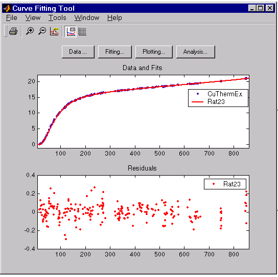
The fit is well behaved over the entire data range, and the residuals are randomly scattered about zero. Therefore, you can confidently use this fit for interpolation and extrapolation.
Example: Gaussian fit
This example fits two poorly resolved Gaussian peaks on a decaying exponential background. To get started, load the data from the gauss3 file:
load gauss3
The workspace contains two new variables:
xpeakis a vector of predictor values.ypeakis a vector of response values.
You will fit the data with the following equation:
\[y(x) = ae^{-bx} + a_{1}e^{ -\left(x - b_{1}\over c_{1} \right) ^2} + a_{2}e^{ -\left(x - b_{2}\over c_{2} \right) ^2}\]where \(a_{i}\) are the peak amplitudes, \(b_{i}\) are the peak centroids, and \(c_{i}\) are related to the peak widths. Since there are unknown coefficients included in the exponential function arguments, the equation is nonlinear. Therefore, you must specify the equation using the General Equations tab of the Create Custom Equation GUI.
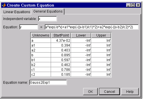
The data, fit, and numerical fit results are shown below. Clearly, the fit is poor. Note that since the starting points are randomly selected, your initial fit results may differ.
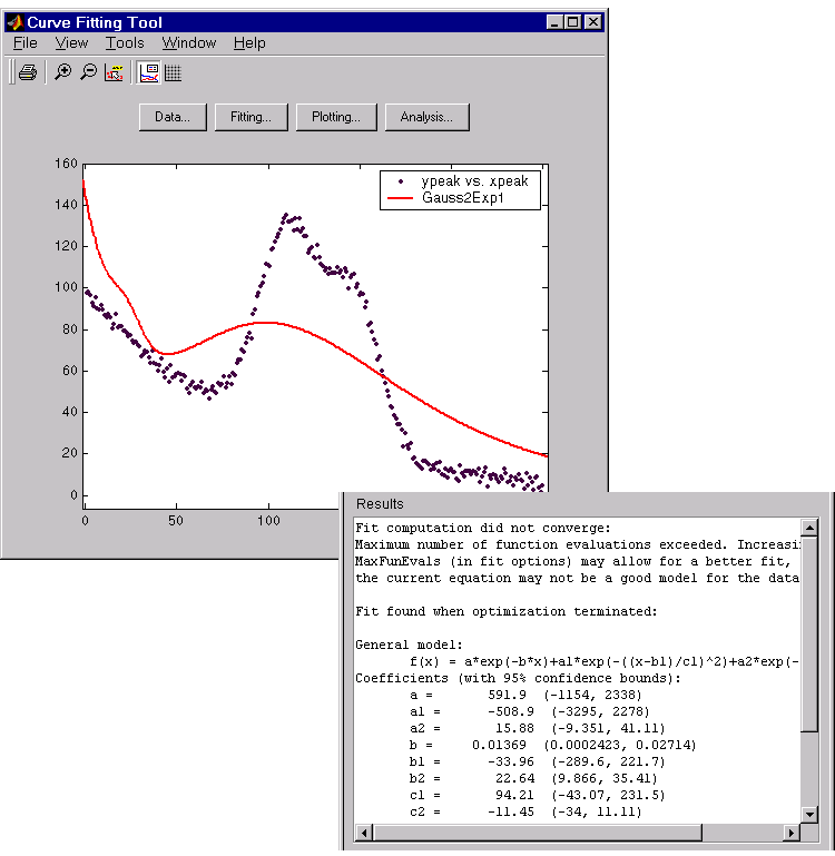
The results include this warning message:
Fit computation did not converge:
Maximum number of function evaluations exceeded. Increasing
MaxFunEvals (in fit options) may allow for a better fit, or
the current equation may not be a good model for the data.
To improve the fit, specify reasonable starting points for the coefficients. Deducing the starting points is particularly easy for the current model since the Gaussian coefficients have a straightforward interpretation and the exponential background is well defined. Additionally, since the peak widths cannot be negative, constrain \(c_{1}\) and \(c_{2}\) to be > 0.
To define starting values and constraints for unknown coefficients, use the Fit Options GUI, which you open by pressing the Fit options button. The starting values and constraints are shown below.
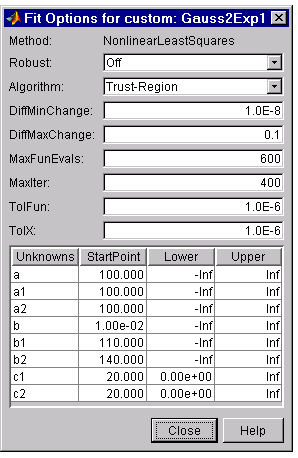
The data, fit, residuals, and numerical results are shown below.

Example: Fourier series fit
This example fits the ENSO data using several custom nonlinear equations. The ENSO data consists of monthly averaged atmospheric pressure differences between Easter Island and Darwin, Australia. This difference drives the trade winds in the southern hemisphere. To get started, load the data from the enso file:
load enso
The ENSO data are periodic, which suggests it can be described by a Fourier series. As a first attempt, assume a 12 month cycle and fit the data using one sine term and one cosine term.
\[y_{1}(x) = a_{0} + a_{1}cos\left(2\pi {x \over c_{1}}\right) + b_{1}sin\left(2\pi {x \over c_{1}}\right)\]If the fit does not describe the data well, add additional sine and cosine terms with unique period coefficients until a good fit is obtained.
Since there is an unknown coefficient \(c_{1}\) included as part of the trigonometric function arguments, the equation is nonlinear. Therefore, you must specify the equation using the General Equations tab of the Create Custom Equation GUI. This tab is shown below for the equation given by \(y_{1}(x)\).

Note that the tool includes the Fourier series as a nonlinear library equation. However, the library equation does not meet the needs of this example since all of its terms are defined as a fixed multiple of the fundamental frequency \(w\).
The numerical results shown below indicate that the fit does not describe the data well. In particular, the fitted value for \(c_{1}\) is unreasonably small. Since the starting points are randomly selected, your initial fit results may differ from the results shown here.

To assist the fitting procedure, constrain \(c_{1}\) to a value between 10 and 14. To define constraints for unknown coefficients, use the Fit Options GUI, which you open by pressing the Fit options button in the Fitting GUI.

The fit, residuals, and numerical results are shown below.
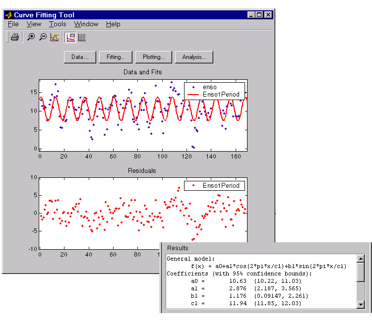
The fit appears to be reasonable for some of the data points but clearly does not describe the entire data set very well. As predicted, the numerical results indicate a cycle of approximately 12 months. However, the residuals show a systematic periodic distribution indicating that there are additional cycles that you should include in the fit equation. Therefore, as a second attempt, add an additional sine and cosine term to \(y_{1}(x)\):
\[y_{2}(x) = y_{1}(x) + a_{2}cos\left(2\pi {x \over c_{1}}\right) + b_{2}sin\left(2\pi {x \over c_{1}}\right)\]and constrain the upper and lower bound of \(c_{2}\) to be roughly twice the bounds used for \(c_{1}\).
The fit, residuals, and numerical results are shown below.
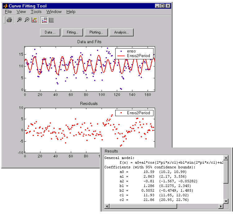
The fit appears to be reasonable for most of the data points. However, the residuals indicate that you should include another cycle to the fit equation. Therefore, as a third attempt, add an additional sine and cosine term to \(y_{2}(x)\)
\[y_{3}(x) = y_{2}(x) + a_{3}cos\left(2\pi {x \over c_{1}}\right) + b_{3}sin\left(2\pi {x \over c_{1}}\right)\]and constrain the lower bound of \(c_{3}\) to be roughly three times the value of \(c_{1}\).
The fit, residuals, and numerical results are shown below.
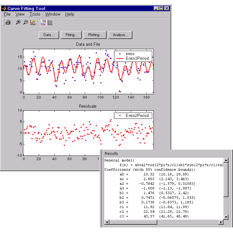
The fit is an improvement over the previous two fits, and appears to account for most of the cycles present in the ENSO data set. The residuals appear random for most of the data, although a pattern is still visible indicating that additional cycles may be present.
In conclusion, Fourier analysis of the data reveals three significant cycles. The annual cycle is the strongest, but cycles with periods of approximately 44 and 22 months are also present. These cycles correspond to El Nino and the Southern Oscillation (ENSO).
Example: Legendre polynomial fit
This example fits generated data using several custom linear equations. The data is based on the nuclear reaction \(^{12}C(e,e'\alpha)^{8}Be\) and the equations use sums of Legendre polynomial terms.
Consider an experiment in which electrons are scattered from 12C nuclei. In the subsequent reaction, alpha particles are emitted and produce the residual nuclei 8Be. By analyzing the number of alpha particles emitted as a function of angle, you can deduce certain information regarding the dynamics of 12C. The reaction kinematics are shown below.
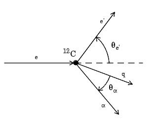
where e is the incident electron, 12C is the carbon target, q is the momentum transfer, e\(^{\prime}\) is the scattered electron, \(\alpha\) is the emitted alpha particle, \(\theta_{e^{\prime}}\) is the electron scattering angle, and \(\theta_{\alpha^{\prime}}\) is the alpha scattering angle.
You can describe a variable expressed as a function of angle in terms of Legendre polynomials:
\[y(x) = \sum_{n=0}^{\infty}a_{n}P_{n}(x)\]where \(P_{n}(x)\) is a Legendre polynomial of degree \(n\), \(x\) is \(\cos(\theta_{\alpha})\), and \(a_{n}\) are the coefficients of the fit.
For the alpha emission data, you can directly associate the coefficients with the nuclear dynamics by invoking a theoretical model. Additionally, the theoretical model introduces constraints for the infinite sum shown above. In particular, by considering the angular momentum of the reaction, a fourth degree Legendre polynomial using only even terms should describe the data effectively.
You can generate Legendre polynomials with Rodrigues’ formula.
\[P_n(x) = {1 \over 2{^n}n!}\left( {d \over dx}\right)^{n}(x^{2} -1)^{n}\]The Legendre polynomials up to fourth degree are given below.
| n | \(P_n(x)\) |
| 0 | 1 |
| 1 | x |
| 2 | \((1/2)(3x^{2}-1)\) |
| 3 | \((1/2)(5x^{3}-3x)\) |
| 4 | \((1/8)(35x^{4}-30x^{2}+3)\) |
The first step is to load the 12C alpha emission data from the carbon12alpha file.
load carbon12alpha
The workspace contains two new variables:
angleis a vector of angles (in radians) ranging from \(10^{\circ}\) to \(240^{\circ}\) in \(10^{\circ}\) increments.countsis a vector of raw alpha particle counts that correspond to the emission angles inangle.
Load these two variables into the Curve Fitting Tool and name the data set C12Alpha.
The Fit Editor for a custom equation fit type is shown below.
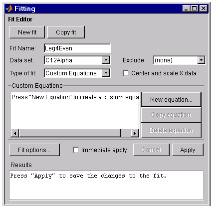
Fit the data using a fourth degree Legendre polynomial with only even terms.
\[y_1(x) = a_0 + a_2{\left(1 \over 2\right)}(3x^{2}-1) + a_4{\left(1 \over 8\right)}(35x^{4}-30x^{2}+3)\]Since the Legendre polynomials depend only on the predictor variable and constants, you use the Linear Equations tab on the Create Custom Equation GUI. This tab is shown below for the model given by \(y_1(x)\). Note that since the angle is given in radians, the argument of the Legendre terms is given by \(cos(\theta_{\alpha})\).

The fit and residuals are shown below. The fit appears to follow the trend of the data, while the residuals appear to be randomly distributed and do not exhibit any systematic behavior.

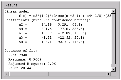
The numerical fit results are shown below. The 95% confidence bounds indicate that the coefficients associated with \(P_0(x)\) and \(P_4(x)\) are known fairly accurately, but that the \(P_2(x)\) coefficient has a relatively large uncertainty.
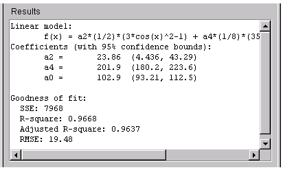
To confirm the theoretical argument that the alpha-emission data is best described by a fourth degree Legendre polynomial with only even terms, fit the data using both even and odd terms.
\[y_2(x) = y_1(x) + a_3 {\left(1 \over 2\right)}(5x^{3}-3x)\]The Linear Equations tab of the Create Custom Equation GUI is shown below for the model given by \(y_2(x)\).
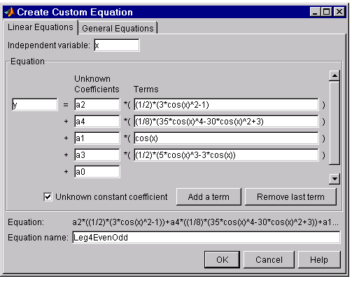
The numerical results indicate that the odd Legendre terms do not contribute significantly to the fit, and the even Legendre terms are essentially unchanged from the previous fit. This confirms that the initial model choice is best.
