Introduction
Curve fitting refers to fitting curved lines to data. The curved line comes from regression techniques, a spline calculation, or interpolation. You can select a predefined model or create your own model. If you do not have a specific model in mind, you can fit using an interpolant or a spline.
The goal of curve fitting is to gain insight into your data. The data can be measured from a sensor, generated from a simulation, historical, and so on. The insight will enable you to improve data acquisition techniques for future experiments, accept or refute a theoretical model, extract physical meaning from fitted coefficients, and draw conclusions about the data’s parent population.
This section describes how to fit data and evaluate the fit results using:
- Parametric fits – Fit your data using parametric models such as polynomials, exponentials, Fourier series, and so on. A parametric fit produces coefficients that describe the data globally, and often have physical meaning.
- Nonparametric fits – Fit your data using nonparametric fit types such as splines and interpolants. A nonparametric fit is useful when you want to fit a smooth curve through your data, and you don’t need to extract or interpret fitted coefficients.
The fitting process
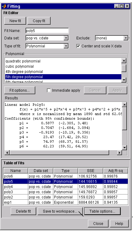
You fit data using the Fitting GUI, which is shown below with the results of a 5th degree polynomial fit of the census data.

The fitting process follows these general steps:
- Specify a fit name - When you press New fit or Copy fit, a default fit name is automatically created. You can specify a new fit name by editing this field.
- Select a data set - Select the name of the data set from the Data set list. All imported and smoothed data sets are listed.
- Select an excluded set - If you want to exclude data from a fit, select an excluded set from the Exclude list. The list contains only excluded sets that are compatible with the selected data set.
- Select a fit type - The fit type can be a library or custom parametric model, a smoothing spline, or an interpolant.
- Specify fit options - Specify fit options such as the fitting algorithm, and coeficient starting points and constraints. Depending on your data and model, accepting the default fit options often produces the best fit.
- Fit the data - Fit the data by pressing the Apply button or by selecting the Immediate apply check box.
- Evaluate the goodness of fit - Examine the fitted curve, residuals, goodness of fit statistics, confidence bounds, and prediction bounds.
- Save results or fit again - If the fit is good, save the results as a structure to the workspace. Otherwise, modify the fit options or select another model.