Syntax
deriv1 = differentiate(fitresult,x)
[deriv1,deriv2] = differentiate(...)
where
fitresult |
A fit result object |
x |
A column vector of values at which fresult is differentiated |
deriv1 |
A column vector of first derivatives |
deriv2 |
A column vector of second derivatives |
Description
deriv1 = differentiate(fitresult,x) differentiates the fit result object fresult at the points specified by x and returns the result to deriv1. You can generate fresult with the fit function or the cfit function.
[deriv1,deriv2] = differentiate(...) computes the first derivative deriv1, and the second derivative deriv2 for the specified fit result object.
For library equations with closed forms, analytic derivatives are calculated. For all other equations, the first derivative is calculated using the central difference quotient.
\[y' = {y_{x+h} - y_{x-h} \over 2h}\]where x is the predictor value at which the derivative is calculated, h is a small number, \(y_{x+h}\) is fresult evaluated at x+h, and \(y_{x-h}\) is fresult evaluated at x-h. The second derivative is calculated using the following expression.
Example
Create a noisy sine wave on the interval [0, 4\(\pi\)].
rand('state',0);
x = linspace(0,4*pi,200)';
y = sin(x) + (rand(size(x))-0.5)*0.2;
Create a custom fit type, and fit the data using reasonable starting values.
ftype = fittype('a*sin(b*x)');
fopts = fitoptions('Method','Nonlinear','start',[1 1]);
fit1 = fit(x,y,ftype,fopts);
Calculate the first derivative for each value of x.
deriv1 = differentiate(fit1,x);
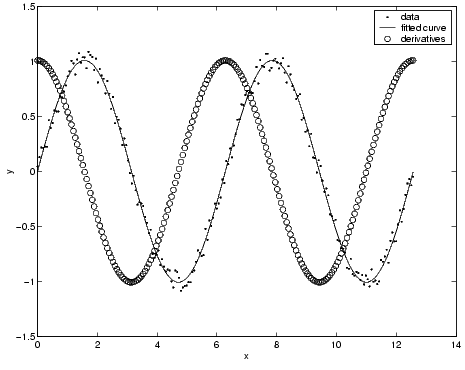
Plot the data, the fit to the data, and the first derivatives.
plot(fit1,'k-',x,y,'b.');hold on
plot(x,deriv1,'ro')
legend('data','fitted curve','derivatives')
