Introduction
If there is justification, you may want to exclude part of a data set from a fit. Typically, you exclude data so that subsequent fits are not adversely affected. For example, if you are fitting a parametric model to measured data that has been corrupted by a faulty sensor, then the resulting fit coefficients will be inaccurate.
The Curve Fitting Tool provides two methods to exclude data:
- Marking outliers – Outliers are defined as individual data points that you exclude because they are inconsistent with the statistical nature of the bulk of the data.
- Sectioning – Sectioning excludes a window of response or predictor data. For example, if many data points in a data set are corrupted by large systematic errors, then you may want to section them out of the fit.
For each of these methods, you must create an excluded set that captures the range, domain, or index of the data points to be excluded.
To exclude data while fitting, you use the Fitting GUI to associate the appropriate excluded set with the data set to be fit. You mark data to be excluded from a fit with the Exclude and Section tab of the Data GUI:
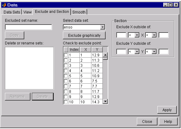
The fields are described below:
- Excluded set name – Specify the name of the excluded set that will identify the data points to be excluded from subsequent fits. You must specify a name before pressing the Apply button.
- Delete or rename sets – Lists the names of all excluded data sets created during the current session. When you select an excluded set, you can perform these actions:
- Press Copy to copy the excluded set. The exclusions associated with the original excluded set are recreated in the GUI. You can modify the exclusions and press Apply to save them to the copied set.
- Press Rename to change the name of the excluded set.
- Press Delete to delete the excluded set.
- Select data set – Select the data set from which data points will be marked as excluded. You must select a data set to exclude individual data points.
-
Exclude graphically – Open a figure window that allows you to exclude individual data points graphically.
The excluded data points are marked by an “x” in the figure, and are identified in the associated table.
- Check to exclude point – Select individual data points to exclude. You can sort this table by clicking on any of the column headings.
- Section – Specify a vertical window, a horizontal window, or a box of data points to include. The excluded data lie outside these windows. You do not need to select a data set to create an excluded set by sectioning.
- Exclude X outside of – Section the predictor data by specifying the domain outside of which data is excluded.
- Exclude Y outside of – Section the response data by specifying the range outside of which data is excluded.
Marking outliers
Outliers are defined as individual data points that you exclude from a fit because they are inconsistent with the statistical nature of the bulk of the data, and will adversely affect the fit results. Outliers are readily identified by a scatter plot of response data versus predictor data.
Marking outliers with the Curve Fitting Tool follows these rules:
-
You must specify a data set before creating an excluded set.
In general, you should use the excluded set only with the specific data set it was based on. However, the toolbox does not prevent you from using the excluded set with another data set provided the size is the same.
-
Using the Data GUI, you can exclude outliers either graphically or numerically.
One of the basic assumptions underlying curve fitting is that the data is statistical in nature and is described by a particular distribution, which is often assumed to be Gaussian. The statistical nature of the data implies that it contains random variations along with a deterministic component.
data = deterministic component + random component
However, your data set may contain one or more data points that are nonstatistical in nature, or are described by a different statistical distribution. These data points may be easy to identify, or they may be buried in the data and difficult to identify.
A nonstatistical process may involve the measurement of a physical variable such as temperature or voltage in which the random variation is negligible compared to the systematic errors. For example, if your sensor calibration is inaccurate, then the data measured with that sensor will be systematically inaccurate. In some cases, you may be able to quantify this nonstatistical data component and correct the data accordingly. However, if the scatter plot reveals that a handful of response values are far removed from neighboring response values, then these data points are considered outliers and should be excluded from the fit. Outliers are usually difficult to explain away. For example, it may be that your sensor experienced a power surge or someone wrote down the wrong number in a log book.
If you decide there is justification, you should mark outliers to be excluded from subsequent fits – especially parametric fits. Removing these data points can have a dramatic effect on the fit results since the fitting process minimizes the square of the residuals. If you do not exclude outliers, then the resulting fit will be poor for a large portion of your data. Conversely, if you do exclude the outliers and choose the appropriate model, then the fit results will be reasonable.
Since outliers can have a significant effect on a fit, they are considered influential data. However, not all influential data points are outliers. For example, your data set can contain valid data points that are far removed from the rest of the data. The data is valid because it is well described by the model used in the fit. The data is influential because its exclusion will dramatically affect the fit results.
Two types of influential data points are shown below for generated data. Also shown are cubic polynomial fits and a robust fit that is resistant to outliers.
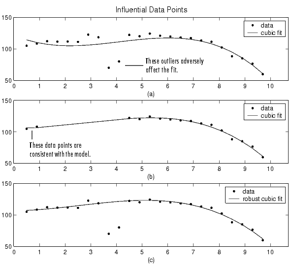
Plot (a) shows that the two influential data points are outliers and adversely affect the fit. Plot (b) shows that the two influential data points are consistent with the model and do not adversely affect the fit. Plot (c) shows that a robust fitting procedure is an acceptable alternative to marking outliers for exclusion.
Sectioning
Sectioning involves specifying a range of response data or a range of predictor data to exclude. You may want to section a data set because different parts of the data set are described by different models or many contiguous data points are corrupted by noise, large systematic errors, and so on.
Sectioning data with the Curve Fitting Tool follows these rules:
-
If you are only sectioning data and not excluding individual data points, then you can create an excluded data set without specifying a data set name.
Note that you can associate the excluded set with any data set provided that the range or domain of the excluded set overlaps with the range or domain of the data set. This is useful if you have multiple data sets from which you want to exclude data points using the same range or domain.
-
Using the Data GUI, you specify a range or domain of data to include. The excluded data lies outside of this specification.
Additionally, you can specify only a single range, domain, or box (range and domain) of included data points. Therefore, at most, you can define two vertical strips, two horizontal strips, or a border of excluded data.
To exclude multiple sections of data, you can use the excludedata function at the MATLAB command line.
Two examples of sectioning by domain are shown below for generated data.
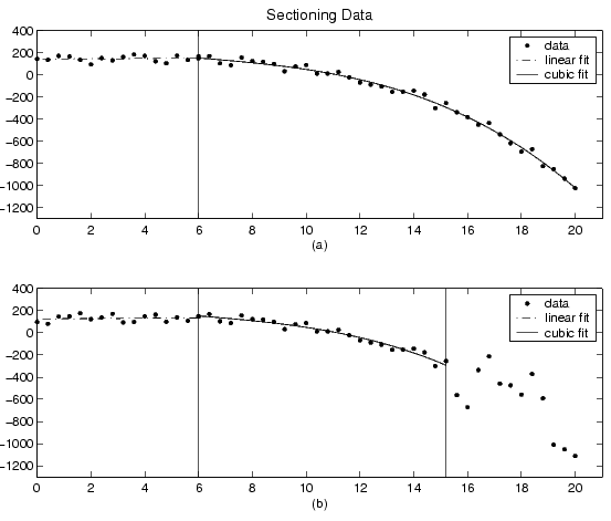
Plot (a) shows the data set sectioned by fit type. The left section is fit with a linear polynomial, while the right section is fit with a cubic polynomial. Plot (b) shows the data set sectioned by fit type and by valid data. Here, the rightmost section is not part of any fit since the data is corrupted by noise. Note that reproducing these plots using the tool is a multistep process. For example, to reproduce plot (a), the steps are:
- Create an excluded set by sectioning the predictor data such that the data points described by the linear polynomial are excluded.
- Create a different excluded set by sectioning the predictor data such that the data points described by the cubic polynomial are excluded.
- Fit the data twice (once for each excluded set) using the appropriate model.
Example: Exclude and section data
This example modifies the ENSO data set to illustrate excluding and sectioning data. First, copy the ENSO response data to a new variable and add two outliers that are far removed from the bulk of the data.
rand('state',0)
yy = pressure;
yy(ceil(length(month)*rand(1))) = mean(pressure)*2.5;
yy(ceil(length(month)*rand(1))) = mean(pressure)*3.0;
Import the variables month and yy as the new data set enso1, and select the Exclude and Section tab of the Data GUI.
Assume that the first and last eight months of the data set are unreliable, and should be excluded from subsequent fits. The simplest way to exclude these data points is to section the predictor data. To do this, specify the range of data you want to include in the Exclude X outside of field of the Section pane.
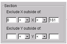
There are two ways to exclude individual data points: using the Check to exclude point table or graphically. For this example, the simplest way to exclude the outliers is graphically. To do this, select the data set name and press the Exclude graphically button, which opens the Select Points for Excluded Set GUI.
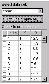
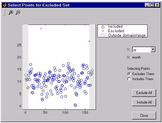
To mark data points for exclusion in the GUI, place the mouse cursor over the data point and left click. The excluded data point is marked with a red X. To include an excluded data point, select the Include Them radio button, place the mouse cursor over the data point and left click. Included data points are marked with a blue circle. To select multiple data points, click the left mouse button and drag the selection rubberband so that it encompasses the desired data points. Note that the GUI identifies sectioned data with gray strips. You cannot graphically include sectioned data.
As shown below, the first and last eight months of data are excluded from the data set by sectioning, and the two outliers are excluded graphically. Note the graphically excluded data points are identified in the Check to exclude point table. If you decide to include an excluded data point using the table, then the graph is automatically updated.
If there are fits associated with the data, you can exclude data points based on the residuals of the fit by selecting the residual data in the Y list.
The Exclude and Section tab for this example is shown below.
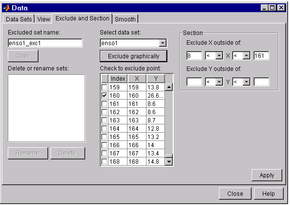
To save the excluded data set, press the Apply button. To exclude the data from a fit, you must select the excluded set from the Exclude list of the Fitting GUI. Since the excluded set created in this example uses individually excluded data points, you can use it only with data sets that are the same size as the ENSO data set.
Viewing the excluded data
There are two ways to view excluded and sectioned data: using the Exclude and Section tab or the View tab:
- Exclude and Section tab – To view an existing excluded set in this tab, you must select the excluded set in the Delete or rename sets list box and press the Copy button. The excluded and sectioned data associated with the original excluded set are recreated in the GUI. You can modify these exclusions and then press Apply to save them to the copied set.
-
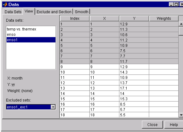
View tab – To view an existing excluded set in this tab, you must select a data set and then select an excluded set. The excluded and sectioned data points are grayed in the table.
An excluded set is compatible with the selected data set if they have the same lengths, or if the excluded set is created by sectioning only.
The View tab displays the modified ENSO data set and the excluded data points, which are grayed in the table.
